Introducción
Se utiliza la librería de sympy para el análisis.
Descargar teoría PDF
Se utiliza la librería de sympy para el análisis.
Descargar teoría PDF
import sympy as sp
# Función para calcular la matriz homogénea
def dh_matrix(a, alpha, d, theta):
return sp.Matrix([
[sp.cos(theta), -sp.sin(theta)*sp.cos(alpha), sp.sin(theta)*sp.sin(alpha), a*sp.cos(theta)],
[sp.sin(theta), sp.cos(theta)*sp.cos(alpha), -sp.cos(theta)*sp.sin(alpha), a*sp.sin(theta)],
[0, sp.sin(alpha), sp.cos(alpha), d],
[0, 0, 0, 1]
])
#dh_matrix(θ, d , a, α)
def reemplazar_trigonometria(matriz, n=3):
"""
Reemplaza las funciones trigonométricas en la matriz:
sin -> S
cos -> C
y evalúa los valores numéricos con 2 decimales.
"""
matriz_reemplazada = matriz.applyfunc(lambda expr: expr.replace(sp.sin, lambda x: sp.Symbol(f'S({x})')).replace(sp.cos, lambda x: sp.Symbol(f'C({x})')))
return matriz_reemplazada.evalf(n)
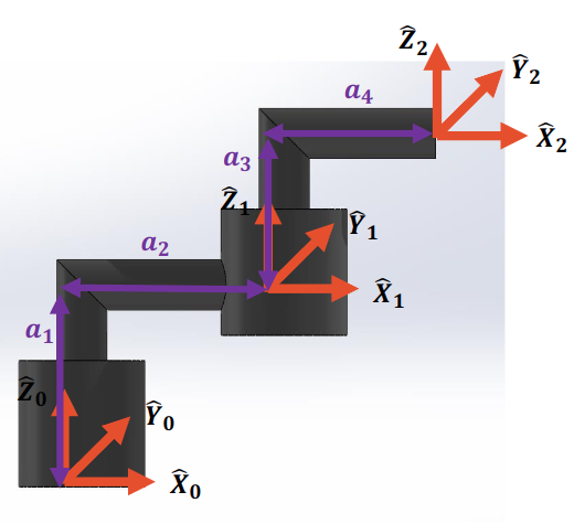
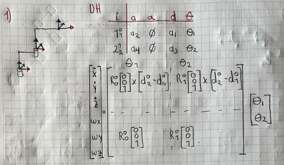
print("\nEjercicio 1: ------------------------------------------------")
# Definir las variables simbólicas
th1, a1, a2, a3, a4, th2 = sp.symbols('th1 a1 a2 a3 a4 th2')
# Primera fila de la tabla DH:
T1 = dh_matrix(a2,0,a1,th1)
# Segunda fila de la tabla DH:
T2 = dh_matrix(a4,0,a3,th2)
# Matriz final: Producto de las transformaciones
T = T1 @ T2
# Mostrar las matrices individuales y el producto final, redondeado a 2 decimales
print("Matriz T1:")
sp.pprint(reemplazar_trigonometria(T1)) # Redondear a 2 decimales
print("\nMatriz T2:")
sp.pprint(reemplazar_trigonometria(T2)) # Redondear a 2 decimales
print("\nMatriz homogénea total T:")
sp.pprint(reemplazar_trigonometria(T)) # Redondear a 2 decimales
# Jacobiano de velocidades
x_v,y_v,z_v,w_x,w_y,w_z = sp.symbols('x_v y_v z_v w_x w_y w_z')
#Vector de velocidades
V = sp.Matrix([x_v, y_v, z_v, w_x, w_y, w_z])
#Obtencion de vector de velocidades lineales th1
R=sp.Matrix([0, 0, 1])
#Tomar solo los valores de la matriz de transformación homogénea
D = T[0:3,3]
Vth1_lin = R.cross(D)
print("\nVector de velocidades lineales th1:")
sp.pprint(Vth1_lin)
#Obtencion de vector de velocidades lineales th2
R=sp.Matrix([0, 0, 1])
D=T[0:3,3]-T1[0:3,3]
Vth2_lin = R.cross(D)
print("\nVector de velocidades lineales th2:")
sp.pprint(Vth2_lin)
#Obtencion de vector de velocidades angulares th1
R=sp.Matrix([0, 0, 1])
Vth1_ang = R
print("\nVector de velocidades angulares th1:")
sp.pprint(Vth1_ang)
#Obtencion de vector de velocidades angulares th2
R=sp.Matrix([0, 0, 1])
Vth2_ang = R
print("\nVector de velocidades angulares th2:")
sp.pprint(Vth2_ang)
#Meterlo en una matriz de 6x2 y multiplicar por el vector de [th1, th2]
V_R=sp.Matrix([
[Vth1_lin[0], Vth2_lin[0]],
[Vth1_lin[1], Vth2_lin[1]],
[Vth1_lin[2], Vth2_lin[2]],
[Vth1_ang[0], Vth2_ang[0]],
[Vth1_ang[1], Vth2_ang[1]],
[Vth1_ang[2], Vth2_ang[2]]
])
th_v = sp.Matrix([th1, th2])
J = V_R @ th_v
#Imprimir el vector de velocidades y el jacobiano equivalente
print("\nVector de velocidades:")
sp.pprint(sp.Eq(V, J))
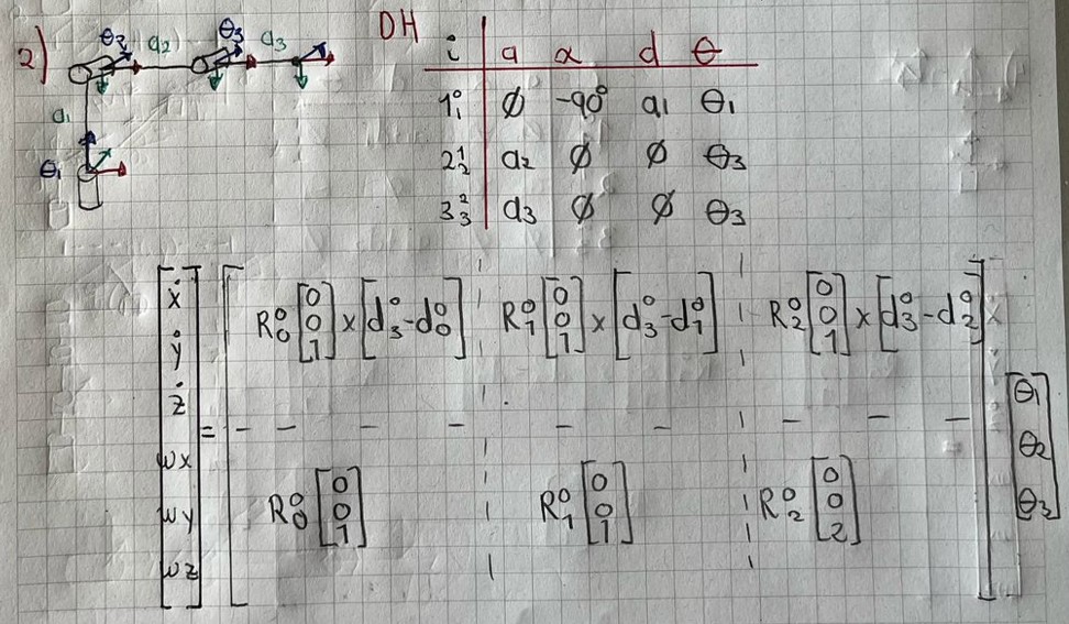
print("\nEjercicio 2: ------------------------------------------------")
# Definir las variables simbólicas
a1, a2, a3, th1, th2, th3 = sp.symbols('a1 a2 a3 th1 th2 th3')
# Primera fila de la tabla DH:
T1 = dh_matrix(0,-sp.pi/2,a1,th1)
# Segunda fila de la tabla DH:
T2 = dh_matrix(a2,0,0,th2)
# Tercera fila de la tabla DH:
T3 = dh_matrix(a3,0,0,th3)
# Matriz final: Producto de las transformaciones
T = T1 @ T2 @ T3
# Mostrar las matrices individuales y el producto final, redondeado a 2 decimales
print("Matriz T1:")
sp.pprint(reemplazar_trigonometria(T1)) # Redondear a 2 decimales
print("\nMatriz T2:")
sp.pprint(reemplazar_trigonometria(T2)) # Redondear a 2 decimales
print("\nMatriz T3:")
sp.pprint(reemplazar_trigonometria(T3)) # Redondear a 2 decimales
print("\nMatriz homogénea total T:")
sp.pprint(reemplazar_trigonometria(T)) # Redondear a 2 dec
# Matriz de 0 a 1
T01 = T1
# Matriz de 0 a 2
T02 = T1 @ T2
# Matriz de 0 a 3
T03 = T
# Jacobiano de velocidades
x_v,y_v,z_v,w_x,w_y,w_z = sp.symbols('x_v y_v z_v w_x w_y w_z')
#Vector de velocidades
V = sp.Matrix([x_v, y_v, z_v, w_x, w_y, w_z])
#Obtencion de vector de velocidades lineales th1
R00=sp.Matrix([0, 0, 1])
#Tomar solo los valores de la matriz de transformación homogénea
D = T[0:3,3]
Vth1_lin = R00.cross(D)
print("\nVector de velocidades lineales th1:")
sp.pprint(Vth1_lin)
#Obtencion de vector de velocidades lineales th2
#Rotacion de T01 por [0,0,1]; extraer matriz de rotacion de T01 homogenea
R01=T01[0:3,0:3]
R01=R01@(sp.Matrix([0, 0, 1]))
# sp.pprint(R)
#Tomar solo los valores de la matriz de transformación homogénea
D=T03[0:3,3]-T01[0:3,3]
Vth2_lin = R01.cross(D)
print("\nVector de velocidades lineales th2:")
sp.pprint(Vth2_lin)
#Obtencion de vector de velocidades lineales th3
#Rotacion de T02 por [0,0,1]; extraer matriz de rotacion de T02 homogenea
R02=T02[0:3,0:3]
R02=R02@(sp.Matrix([0, 0, 1]))
# sp.pprint(R)
#Tomar solo los valores de la matriz de transformación homogénea
D=T03[0:3,3]-T02[0:3,3]
Vth3_lin = R02.cross(D)
print("\nVector de velocidades lineales th3:")
sp.pprint(Vth3_lin)
#Obtencion de vector de velocidades angulares th1
#R00
print("\nVector de velocidades angulares th1:")
sp.pprint(R00)
Vth1_ang = R00
#Obtencion de vector de velocidades angulares th2
#R01
print("\nVector de velocidades angulares th2:")
sp.pprint(R01)
Vth2_ang = R01
#Obtencion de vector de velocidades angulares th3
#R02
print("\nVector de velocidades angulares th3:")
sp.pprint(R02)
Vth3_ang = R02
#Meterlo en una matriz de 6x3 y multiplicar por el vector de [th1, th2, th3]
V_R=sp.Matrix([
[Vth1_lin[0], Vth2_lin[0], Vth3_lin[0]],
[Vth1_lin[1], Vth2_lin[1], Vth3_lin[1]],
[Vth1_lin[2], Vth2_lin[2], Vth3_lin[2]],
[Vth1_ang[0], Vth2_ang[0], Vth3_ang[0]],
[Vth1_ang[1], Vth2_ang[1], Vth3_ang[1]],
[Vth1_ang[2], Vth2_ang[2], Vth3_ang[2]]
])
th_v = sp.Matrix([th1, th2, th3])
J = V_R @ th_v
#Imprimir el vector de velocidades y el jacobiano equivalente
print("\nVector de velocidades:")
sp.pprint(sp.Eq(V, J))
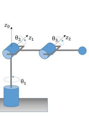
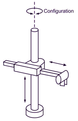
print("\nEjercicio 3: ------------------------------------------------")
# Definir las variables simbólicas
a1, a2, d1, th1, th2 = sp.symbols('a1 a2 d1 th1 th2')
# Primera fila de la tabla DH:
T1 = dh_matrix(0,-sp.pi/2,a1,th1)
# Segunda fila de la tabla DH:
T2 = dh_matrix(0,-sp.pi/2,0,th2)
# Tercera fila de la tabla DH:
T3 = dh_matrix(0,0,a2+d1,0)
# Matriz final: Producto de las transformaciones
T = T1 @ T2 @ T3
# Mostrar las matrices individuales y el producto final, redondeado a 2 decimales
print("Matriz T1:")
sp.pprint(reemplazar_trigonometria(T1)) # Redondear a 2 decimales
print("\nMatriz T2:")
sp.pprint(reemplazar_trigonometria(T2)) # Redondear a 2 decimales
print("\nMatriz T3:")
sp.pprint(reemplazar_trigonometria(T3)) # Redondear a 2 decimales
print("\nMatriz homogénea total T:")
sp.pprint(reemplazar_trigonometria(T)) # Redondear a 2 decimales
# Matriz de 0 a 1
T01 = T1
# Matriz de 0 a 2
T02 = T1 @ T2
# Matriz de 0 a 3
T03 = T
#Jacobiano de velocidades
x_v,y_v,z_v,w_x,w_y,w_z = sp.symbols('x_v y_v z_v w_x w_y w_z')
#Vector de velocidades
V = sp.Matrix([x_v, y_v, z_v, w_x, w_y, w_z])
#Obtencion de vector de velocidades lineales th1
R00=sp.Matrix([0, 0, 1])
#Tomar solo los valores de la matriz de transformación homogénea
D = T[0:3,3]
Vth1_lin = R00.cross(D)
print("\nVector de velocidades lineales th1:")
sp.pprint(Vth1_lin)
#Obtencion de vector de velocidades lineales th2
#Rotacion de T01 por [0,0,1]; extraer matriz de rotacion de T01 homogenea
R01=T01[0:3,0:3]
R01=R01@(sp.Matrix([0, 0, 1]))
# sp.pprint(R)
#Tomar solo los valores de la matriz de transformación homogénea
D=T03[0:3,3]-T01[0:3,3]
Vth2_lin = R01.cross(D)
print("\nVector de velocidades lineales th2:")
sp.pprint(Vth2_lin)
#Obtencion de vector de velocidades lineales d1
R02=T02[0:3,0:3]
R02=R02@(sp.Matrix([0, 0, 1]))
Vd1_lin = R02
print("\nVector de velocidades lineales d1:")
sp.pprint(Vd1_lin)
#Obtencion de vector de velocidades angulares th1
#R00
print("\nVector de velocidades angulares th1:")
sp.pprint(R00)
Vth1_ang = R00
#Obtencion de vector de velocidades angulares th2
#R01
print("\nVector de velocidades angulares th2:")
sp.pprint(R01)
Vth2_ang = R01
#Obtencion de vector de velocidades angulares d1
#Traslacional no tiene velocidad angular
Vd1_ang = sp.Matrix([0, 0, 0])
print("\nVector de velocidades angulares d1:")
sp.pprint(Vd1_ang)
#Meterlo en una matriz de 6x3 y multiplicar por el vector de [th1, th2, d1]
V_R=sp.Matrix([
[Vth1_lin[0], Vth2_lin[0], Vd1_lin[0]],
[Vth1_lin[1], Vth2_lin[1], Vd1_lin[1]],
[Vth1_lin[2], Vth2_lin[2], Vd1_lin[2]],
[Vth1_ang[0], Vth2_ang[0], Vd1_ang[0]],
[Vth1_ang[1], Vth2_ang[1], Vd1_ang[1]],
[Vth1_ang[2], Vth2_ang[2], Vd1_ang[2]]
])
th_v = sp.Matrix([th1, th2, d1])
J = V_R @ th_v
#Imprimir el vector de velocidades y el jacobiano equivalente
print("\nVector de velocidades:")
sp.pprint(sp.Eq(V, J))
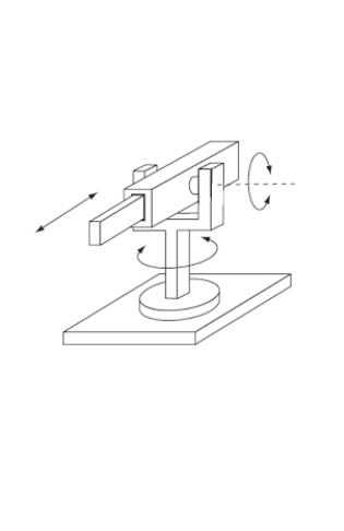
print("\nEjercicio 4: ------------------------------------------------")
# Definir las variables simbólicas
a1, a2, a3, d1, d2, th1 = sp.symbols('a1 a2 a3 d1 d2 th1')
# Primera fila de la tabla DH:
T1 = dh_matrix(0,0,a1+d1,0)
# Segunda fila de la tabla DH:
T2 = dh_matrix(a2,sp.pi/2,0,th1)
# Tercera fila de la tabla DH:
T3 = dh_matrix(0,0,a3+d2,0)
# Matriz final: Producto de las transformaciones
T = T1 @ T2 @ T3
# Mostrar las matrices individuales y el producto final, redondeado a 2 decimales
print("Matriz T1:")
sp.pprint(reemplazar_trigonometria(T1)) # Redondear a 2 decimales
print("\nMatriz T2:")
sp.pprint(reemplazar_trigonometria(T2)) # Redondear a 2 decimales
print("\nMatriz T3:")
sp.pprint(reemplazar_trigonometria(T3)) # Redondear a 2 decimales
print("\nMatriz homogénea total T:")
sp.pprint(reemplazar_trigonometria(T)) # Redondear a 2 decimales
# Matriz de 0 a 1
T01 = T1
# Matriz de 0 a 2
T02 = T1 @ T2
# Matriz de 0 a 3
T03 = T
#Jacobiano de velocidades
x_v,y_v,z_v,w_x,w_y,w_z = sp.symbols('x_v y_v z_v w_x w_y w_z')
#Vector de velocidades
V = sp.Matrix([x_v, y_v, z_v, w_x, w_y, w_z])
#Obtencion de vector de velocidades lineales d1
R00=sp.Matrix([0, 0, 1])
#Prismático
Vd1_lin = R00
print("\nVector de velocidades lineales d1:")
sp.pprint(Vd1_lin)
#Obtencion de vector de velocidades lineales th1
#Rotacion de T01 por [0,0,1]; extraer matriz de rotacion de T01 homogenea
R01=T01[0:3,0:3]
R01=R01@(sp.Matrix([0, 0, 1]))
#Tomar solo los valores de la matriz de transformación homogénea
D=T03[0:3,3]-T01[0:3,3]
Vth1_lin = R01.cross(D)
print("\nVector de velocidades lineales th1:")
sp.pprint(Vth1_lin)
#Obtencion de vector de velocidades lineales d2
R02=T02[0:3,0:3]
R02=R02@(sp.Matrix([0, 0, 1]))
#Primatico
Vd2_lin = R02
print("\nVector de velocidades lineales d2:")
sp.pprint(Vd2_lin)
#Obtencion de vector de velocidades angulares d1
#Primático no tiene rotación
Vd1_ang = sp.Matrix([0, 0, 0])
print("\nVector de velocidades angulares d1:")
sp.pprint(Vd1_ang)
#Obtencion de vector de velocidades angulares th1
#R01
print("\nVector de velocidades angulares th1:")
Vth1_ang = R01
sp.pprint(Vth1_ang)
#Obtencion de vector de velocidades angulares d2
#Primático no tiene rotación
Vd2_ang = sp.Matrix([0, 0, 0])
print("\nVector de velocidades angulares d2:")
sp.pprint(Vd2_ang)
#Meterlo en una matriz de 6x3 y multiplicar por el vector de [d1, th1, d2]
V_R=sp.Matrix([
[Vd1_lin[0], Vth1_lin[0], Vd2_lin[0]],
[Vd1_lin[1], Vth1_lin[1], Vd2_lin[1]],
[Vd1_lin[2], Vth1_lin[2], Vd2_lin[2]],
[Vd1_ang[0], Vth1_ang[0], Vd2_ang[0]],
[Vd1_ang[1], Vth1_ang[1], Vd2_ang[1]],
[Vd1_ang[2], Vth1_ang[2], Vd2_ang[2]]
])
th_v = sp.Matrix([d1, th1, d2])
J = V_R @ th_v
#Imprimir el vector de velocidades y el jacobiano equivalente
print("\nVector de velocidades:")
sp.pprint(sp.Eq(V, J))
⎡C(th1)  -S(th1)   0   C(th1)⋅a₂ ⎤
⎢                               ⎥
⎢S(th1)  C(th1)    0   S(th1)⋅a₂⎥
⎢                               ⎥
⎢  0        0     1.0     a₁    ⎥
⎢                               ⎥
⎣  0        0      0      1.0   ⎦
⎡C(th2)  -S(th2)   0   C(th2)⋅a₄⎤
⎢                               ⎥
⎢S(th2)  C(th2)    0   S(th2)⋅a₄⎥
⎢                               ⎥
⎢  0        0     1.0     a₃    ⎥
⎢                               ⎥
⎣  0        0      0      1.0   ⎦
⎡C(th1)⋅C(th2) - S(th1)⋅S(th2)  -C(th1)⋅S(th2) - C(th2)⋅S(th1)   0   C(th1)⋅C(th2)⋅a₄ + C(th1)⋅a₂ - S(th1)⋅S(th2)⋅a₄     ⎤
⎢                                                                                                                   ⎥
⎢C(th1)⋅S(th2) + C(th2)⋅S(th1)  C(th1)⋅C(th2) - S(th1)⋅S(th2)    0   C(th1)⋅S(th2)⋅a₄ + C(th2)⋅S(th1)⋅a₄ + S(th1)⋅a₂     ⎥
⎢                                                                                                                   ⎥
⎢              0                              0                 1.0                      a₁ + a₃                    ⎥
⎢                                                                                                                   ⎥
⎣              0                              0                  0                         1.0                      ⎦
⎡-a₂⋅sin(th₁) - a₄⋅sin(th₁)⋅cos(th₂) - a₄⋅sin(th₂)⋅cos(th₁)   ⎤
⎢                                                          ⎥
⎢a₂⋅cos(th₁) - a₄⋅sin(th₁)⋅sin(th₂) + a₄⋅cos(th₁)⋅cos(th₂)    ⎥
⎢                                                          ⎥
⎣                            0                             ⎦
⎡-a₄⋅sin(th₁)⋅cos(th₂) - a₄⋅sin(th₂)⋅cos(th₁)   ⎤
⎢                                            ⎥
⎢-a₄⋅sin(th₁)⋅sin(th₂) + a₄⋅cos(th₁)⋅cos(th₂)   ⎥
⎢                                            ⎥
⎣                     0                      ⎦
⎡0⎤
⎢ ⎥
⎢0⎥
⎢ ⎥
⎣1⎦
⎡0⎤
⎢ ⎥
⎢0⎥
⎢ ⎥
⎣1⎦
⎡xᵥ ⎤   ⎡th₁⋅(-a₂⋅sin(th₁) - a₄⋅sin(th₁)⋅cos(th₂) - a₄⋅sin(th₂)⋅cos(th₁)) + th₂⋅(-a₄⋅sin(th₁)⋅cos(th₂) - a₄⋅sin(th₂)⋅cos(th₁))      ⎤
⎢   ⎥   ⎢                                                                                                                     ⎥
⎢yᵥ ⎥   ⎢th₁⋅(a₂⋅cos(th₁) - a₄⋅sin(th₁)⋅sin(th₂) + a₄⋅cos(th₁)⋅cos(th₂)) + th₂⋅(-a₄⋅sin(th₁)⋅sin(th₂) + a₄⋅cos(th₁)⋅cos(th₂))       ⎥
⎢   ⎥   ⎢                                                                                                                     ⎥
⎢zᵥ ⎥   ⎢                                                          0                                                          ⎥
⎢   ⎥ = ⎢                                                                                                                     ⎥
⎢wₓ ⎥   ⎢                                                          0                                                          ⎥
⎢   ⎥   ⎢                                                                                                                     ⎥
⎢w_y⎥   ⎢                                                          0                                                          ⎥
⎢   ⎥   ⎢                                                                                                                     ⎥
⎣w_z⎦   ⎣                                                      th₁ + th₂                                                      ⎦
⎡C(th1)   0    -S(th1)   0 ⎤
⎢                          ⎥
⎢S(th1)   0    C(th1)    0 ⎥
⎢                          ⎥
⎢  0     -1.0     0     a₁ ⎥
⎢                          ⎥
⎣  0      0       0     1.0⎦
⎡C(th2)  -S(th2)   0   C(th2)⋅a₂⎤
⎢                               ⎥
⎢S(th2)  C(th2)    0   S(th2)⋅a₂⎥
⎢                               ⎥
⎢  0        0     1.0      0    ⎥
⎢                               ⎥
⎣  0        0      0      1.0   ⎦
⎡C(th3)  -S(th3)   0   C(th3)⋅a₃⎤
⎢                               ⎥
⎢S(th3)  C(th3)    0   S(th3)⋅a₃⎥
⎢                               ⎥
⎢  0        0     1.0      0    ⎥
⎢                               ⎥
⎣  0        0      0      1.0   ⎦
⎡C(th1)⋅C(th2)⋅C(th3) - C(th1)⋅S(th2)⋅S(th3)  -C(th1)⋅C(th2)⋅S(th3) - C(th1)⋅C(th3)⋅S(th2)  -S(th1)  C(th1)⋅C(th2)⋅C(th3)⋅a₃ + C(th1)⋅C(th2)⋅a₂ - C(th1)⋅S(th2)⋅S(th3)⋅a₃        ⎤
⎢                                                                                                                                                                        ⎥
⎢C(th2)⋅C(th3)⋅S(th1) - S(th1)⋅S(th2)⋅S(th3)  -C(th2)⋅S(th1)⋅S(th3) - C(th3)⋅S(th1)⋅S(th2)  C(th1)   C(th2)⋅C(th3)⋅S(th1)⋅a₃ + C(th2)⋅S(th1)⋅a₂ - S(th1)⋅S(th2)⋅S(th3)⋅a₃        ⎥
⎢                                                                                                                                                                        ⎥
⎢      -C(th2)⋅S(th3) - C(th3)⋅S(th2)                -C(th2)⋅C(th3) + S(th2)⋅S(th3)            0            -C(th2)⋅S(th3)⋅a₃ - C(th3)⋅S(th2)⋅a₃ - S(th2)⋅a₂ + a₁             ⎥
⎢                                                                                                                                                                        ⎥
⎣                     0                                            0                           0                                     1.0                                 ⎦
⎡-a₂⋅sin(th₁)⋅cos(th₂) + a₃⋅sin(th₁)⋅sin(th₂)⋅sin(th₃) - a₃⋅sin(th₁)⋅cos(th₂)⋅cos(th₃)    ⎤
⎢                                                                                     ⎥
⎢a₂⋅cos(th₁)⋅cos(th₂) - a₃⋅sin(th₂)⋅sin(th₃)⋅cos(th₁) + a₃⋅cos(th₁)⋅cos(th₂)⋅cos(th₃)     ⎥
⎢                                                                                     ⎥
⎣                                          0                                          ⎦
⎡                                                              (-a₂⋅sin(th₂) - a₃⋅sin(th₂)⋅cos(th₃) - a₃⋅sin(th₃)⋅cos(th₂))⋅cos(th₁)                                                                  ⎤
⎢                                                                                                                                                                                                  ⎥
⎢                                                              (-a₂⋅sin(th₂) - a₃⋅sin(th₂)⋅cos(th₃) - a₃⋅sin(th₃)⋅cos(th₂))⋅sin(th₁)                                                                  ⎥
⎢                                                                                                                                                                                                  ⎥
⎣-(a₂⋅sin(th₁)⋅cos(th₂) - a₃⋅sin(th₁)⋅sin(th₂)⋅sin(th₃) + a₃⋅sin(th₁)⋅cos(th₂)⋅cos(th₃))⋅sin(th₁) - (a₂⋅cos(th₁)⋅cos(th₂) - a₃⋅sin(th₂)⋅sin(th₃)⋅cos(th₁) + a₃⋅cos(th₁)⋅cos(th₂)⋅cos(th₃))⋅cos(th₁)         ⎦
⎡                                               (-a₃⋅sin(th₂)⋅cos(th₃) - a₃⋅sin(th₃)⋅cos(th₂))⋅cos(th₁)                                                ⎤
⎢                                                                                                                                                    ⎥
⎢                                               (-a₃⋅sin(th₂)⋅cos(th₃) - a₃⋅sin(th₃)⋅cos(th₂))⋅sin(th₁)                                                ⎥
⎢                                                                                                                                                    ⎥
⎣-(-a₃⋅sin(th₁)⋅sin(th₂)⋅sin(th₃) + a₃⋅sin(th₁)⋅cos(th₂)⋅cos(th₃))⋅sin(th₁) - (-a₃⋅sin(th₂)⋅sin(th₃)⋅cos(th₁) + a₃⋅cos(th₁)⋅cos(th₂)⋅cos(th₃))⋅cos(th₁)     ⎦
⎡0⎤
⎢ ⎥
⎢0⎥
⎢ ⎥
⎣1⎦
⎡-sin(th₁)⎤
⎢         ⎥
⎢cos(th₁) ⎥
⎢         ⎥
⎣    0    ⎦
⎡-sin(th₁)⎤
⎢         ⎥
⎢cos(th₁) ⎥
⎢         ⎥
⎣    0    ⎦
⎡xᵥ ⎤   ⎡                                                                 th₁⋅(-a₂⋅sin(th₁)⋅cos(th₂) + a₃⋅sin(th₁)⋅sin(th₂)⋅sin(th₃) - a₃⋅sin(th₁)⋅cos(th₂)⋅cos(th₃)) + th₂⋅(-a₂⋅sin(th₂) - a₃⋅sin(th₂)⋅cos(th₃) - a₃⋅sin(th₃)⋅cos(th₂))⋅cos(th₁) + th₃⋅(-a₃⋅sin(th₂)⋅cos(th₃) - a₃⋅sin(th₃)⋅cos(th₂))⋅cos(th₁)                                                                            ⎤
⎢   ⎥   ⎢                                                                                                                                                                                                                                                                                                                                                                       ⎥
⎢yᵥ ⎥   ⎢                                                                 th₁⋅(a₂⋅cos(th₁)⋅cos(th₂) - a₃⋅sin(th₂)⋅sin(th₃)⋅cos(th₁) + a₃⋅cos(th₁)⋅cos(th₂)⋅cos(th₃)) + th₂⋅(-a₂⋅sin(th₂) - a₃⋅sin(th₂)⋅cos(th₃) - a₃⋅sin(th₃)⋅cos(th₂))⋅sin(th₁) + th₃⋅(-a₃⋅sin(th₂)⋅cos(th₃) - a₃⋅sin(th₃)⋅cos(th₂))⋅sin(th₁)                                                                             ⎥
⎢   ⎥   ⎢                                                                                                                                                                                                                                                                                                                                                                       ⎥
⎢zᵥ ⎥   ⎢th₂⋅(-(a₂⋅sin(th₁)⋅cos(th₂) - a₃⋅sin(th₁)⋅sin(th₂)⋅sin(th₃) + a₃⋅sin(th₁)⋅cos(th₂)⋅cos(th₃))⋅sin(th₁) - (a₂⋅cos(th₁)⋅cos(th₂) - a₃⋅sin(th₂)⋅sin(th₃)⋅cos(th₁) + a₃⋅cos(th₁)⋅cos(th₂)⋅cos(th₃))⋅cos(th₁)) + th₃⋅(-(-a₃⋅sin(th₁)⋅sin(th₂)⋅sin(th₃) + a₃⋅sin(th₁)⋅cos(th₂)⋅cos(th₃))⋅sin(th₁) - (-a₃⋅sin(th₂)⋅sin(th₃)⋅cos(th₁) + a₃⋅cos(th₁)⋅cos(th₂)⋅cos(th₃))⋅cos(th₁))                 ⎥
⎢   ⎥ = ⎢                                                                                                                                                                                                                                                                                                                                                                       ⎥
⎢wₓ ⎥   ⎢                                                                                                                                                                     -th₂⋅sin(th₁) - th₃⋅sin(th₁)                                                                                                                                                                       ⎥
⎢   ⎥   ⎢                                                                                                                                                                                                                                                                                                                                                                       ⎥
⎢w_y⎥   ⎢                                                                                                                                                                      th₂⋅cos(th₁) + th₃⋅cos(th₁)                                                                                                                                                                       ⎥
⎢   ⎥   ⎢                                                                                                                                                                                                                                                                                                                                                                       ⎥
⎣w_z⎦   ⎣                                                                                                                                                                                  th₁                                                                                                                                                                                  ⎦

⎡C(th1)   0    -S(th1)   0 ⎤
⎢                          ⎥
⎢S(th1)   0    C(th1)    0 ⎥
⎢                          ⎥
⎢  0     -1.0     0     a₁ ⎥
⎢                          ⎥
⎣  0      0       0     1.0⎦
⎡C(th2)   0    -S(th2)   0 ⎤
⎢                          ⎥
⎢S(th2)   0    C(th2)    0 ⎥
⎢                          ⎥
⎢  0     -1.0     0      0 ⎥
⎢                          ⎥
⎣  0      0       0     1.0⎦
⎡1.0   0    0      0   ⎤
⎢                      ⎥
⎢ 0   1.0   0      0   ⎥
⎢                      ⎥
⎢ 0    0   1.0  a₂ + d₁⎥
⎢                      ⎥
⎣ 0    0    0     1.0  ⎦
⎡C(th1)⋅C(th2)  S(th1)   -C(th1)⋅S(th2)  -C(th1)⋅S(th2)⋅(a₂ + d₁)  ⎤
⎢                                                                ⎥
⎢C(th2)⋅S(th1)  -C(th1)  -S(th1)⋅S(th2)  -S(th1)⋅S(th2)⋅(a₂ + d₁)  ⎥
⎢                                                                ⎥
⎢   -S(th2)        0        -C(th2)       -C(th2)⋅(a₂ + d₁) + a₁  ⎥
⎢                                                                ⎥
⎣      0           0           0                   1.0           ⎦
⎡(a₂ + d₁)⋅sin(th₁)⋅sin(th₂)  ⎤
⎢                            ⎥
⎢-(a₂ + d₁)⋅sin(th₂)⋅cos(th₁) ⎥
⎢                            ⎥
⎣             0              ⎦
⎡               -(a₂ + d₁)⋅cos(th₁)⋅cos(th₂)                 ⎤
⎢                                                           ⎥
⎢               -(a₂ + d₁)⋅sin(th₁)⋅cos(th₂)                 ⎥
⎢                                                           ⎥
⎢             2                                       2     ⎥
⎣(a₂ + d₁)⋅sin (th₁)⋅sin(th₂) + (a₂ + d₁)⋅sin(th₂)⋅cos (th₁)  ⎦
⎡-sin(th₂)⋅cos(th₁)⎤
⎢                  ⎥
⎢-sin(th₁)⋅sin(th₂)⎥
⎢                  ⎥
⎣    -cos(th₂)     ⎦
⎡0⎤
⎢ ⎥
⎢0⎥
⎢ ⎥
⎣1⎦
⎡-sin(th₁)⎤
⎢         ⎥
⎢cos(th₁) ⎥
⎢         ⎥
⎣    0    ⎦
⎡0⎤
⎢ ⎥
⎢0⎥
⎢ ⎥
⎣0⎦
       ⎡-d₁⋅sin(th₂)⋅cos(th₁) + th₁⋅(a₂ + d₁)⋅sin(th₁)⋅sin(th₂) - th₂⋅(a₂ + d₁)⋅cos(th₁)⋅cos(th₂)    ⎤
⎡xᵥ ⎤   ⎢                                                                                         ⎥
⎢   ⎥   ⎢-d₁⋅sin(th₁)⋅sin(th₂) - th₁⋅(a₂ + d₁)⋅sin(th₂)⋅cos(th₁) - th₂⋅(a₂ + d₁)⋅sin(th₁)⋅cos(th₂)    ⎥
⎢yᵥ ⎥   ⎢                                                                                         ⎥
⎢   ⎥   ⎢                       ⎛             2                                       2     ⎞     ⎥
⎢zᵥ ⎥   ⎢    -d₁⋅cos(th₂) + th₂⋅⎝(a₂ + d₁)⋅sin (th₁)⋅sin(th₂) + (a₂ + d₁)⋅sin(th₂)⋅cos (th₁)⎠       ⎥
⎢   ⎥ = ⎢                                                                                         ⎥
⎢wₓ ⎥   ⎢                                      -th₂⋅sin(th₁)                                      ⎥
⎢   ⎥   ⎢                                                                                         ⎥
⎢w_y⎥   ⎢                                      th₂⋅cos(th₁)                                       ⎥
⎢   ⎥   ⎢                                                                                         ⎥
⎣w_z⎦   ⎣                                           th₁                                           ⎦

⎡1.0   0    0      0   ⎤
⎢                      ⎥
⎢ 0   1.0   0      0   ⎥
⎢                      ⎥
⎢ 0    0   1.0  a₁ + d₁⎥
⎢                      ⎥
⎣ 0    0    0     1.0  ⎦
⎡C(th1)   0   S(th1)   C(th1)⋅a₂ ⎤
⎢                               ⎥
⎢S(th1)   0   -C(th1)  S(th1)⋅a₂ ⎥
⎢                               ⎥
⎢  0     1.0     0         0    ⎥
⎢                               ⎥
⎣  0      0      0        1.0   ⎦
⎡1.0   0    0      0   ⎤
⎢                      ⎥
⎢ 0   1.0   0      0   ⎥
⎢                      ⎥
⎢ 0    0   1.0  a₃ + d₂⎥
⎢                      ⎥
⎣ 0    0    0     1.0  ⎦
⎡C(th1)   0   S(th1)   C(th1)⋅a₂ + S(th1)⋅(a₃ + d₂)  ⎤
⎢                                                   ⎥
⎢S(th1)   0   -C(th1)  -C(th1)⋅(a₃ + d₂) + S(th1)⋅a₂ ⎥
⎢                                                   ⎥
⎢  0     1.0     0                a₁ + d₁           ⎥
⎢                                                   ⎥
⎣  0      0      0                  1.0             ⎦
⎡0⎤
⎢ ⎥
⎢0⎥
⎢ ⎥
⎣1⎦
⎡-a₂⋅sin(th₁) + (a₃ + d₂)⋅cos(th₁) ⎤
⎢                                 ⎥
⎢a₂⋅cos(th₁) + (a₃ + d₂)⋅sin(th₁)  ⎥
⎢                                 ⎥
⎣                0                ⎦
⎡sin(th₁) ⎤
⎢         ⎥
⎢-cos(th₁)⎥
⎢         ⎥
⎣    0    ⎦
⎡0⎤
⎢ ⎥
⎢0⎥
⎢ ⎥
⎣0⎦
⎡0⎤
⎢ ⎥
⎢0⎥
⎢ ⎥
⎣1⎦
⎡0⎤
⎢ ⎥
⎢0⎥
⎢ ⎥
⎣0⎦
⎡xᵥ ⎤   ⎡d₂⋅sin(th₁) + th₁⋅(-a₂⋅sin(th₁) + (a₃ + d₂)⋅cos(th₁))  ⎤
⎢   ⎥   ⎢                                                     ⎥
⎢yᵥ ⎥   ⎢-d₂⋅cos(th₁) + th₁⋅(a₂⋅cos(th₁) + (a₃ + d₂)⋅sin(th₁))  ⎥
⎢   ⎥   ⎢                                                     ⎥
⎢zᵥ ⎥   ⎢                         d₁                          ⎥
⎢   ⎥ = ⎢                                                     ⎥
⎢wₓ ⎥   ⎢                          0                          ⎥
⎢   ⎥   ⎢                                                     ⎥
⎢w_y⎥   ⎢                          0                          ⎥
⎢   ⎥   ⎢                                                     ⎥
⎣w_z⎦   ⎣                         th₁                         ⎦