Introducción
Se utiliza la librería de python-roboticstoolbox para el análisis.
Descargar teoría PDF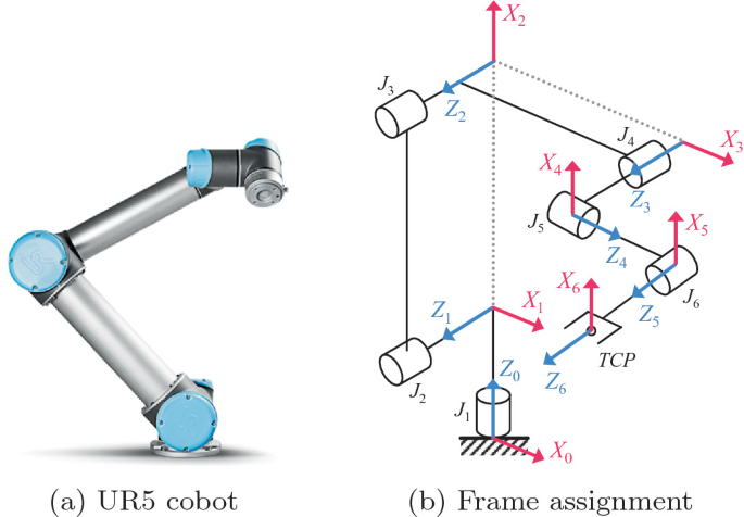
Se utiliza la librería de python-roboticstoolbox para el análisis.
Descargar teoría PDF
import roboticstoolbox as rtb
from spatialmath import SE3
import numpy as np
import matplotlib.pyplot as plt
import sympy as sp
Status_block = False
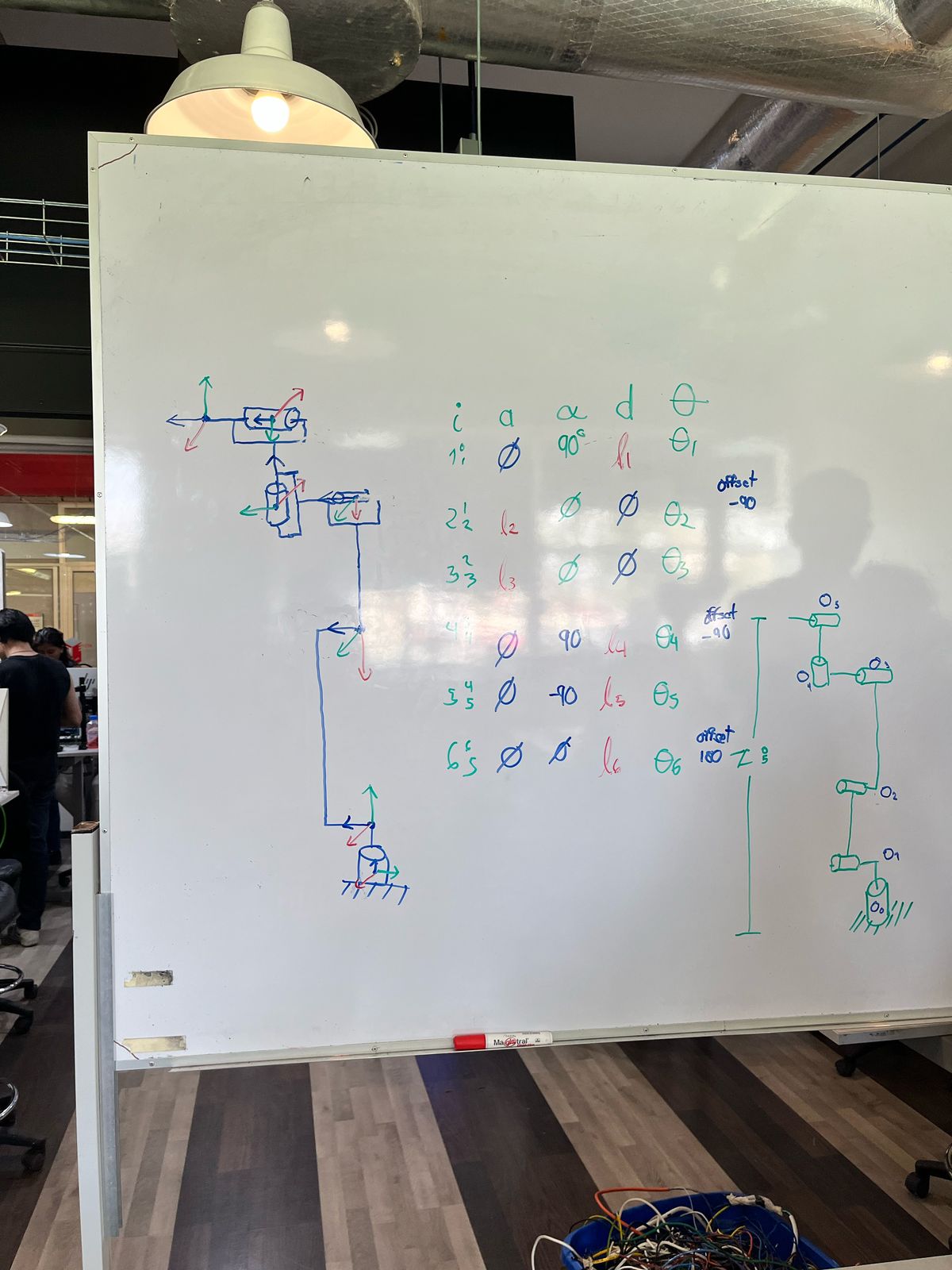
# Robot UR5 --------------------------------------------------------------
name = "UR5"
a1 = 0.1625
a2 = 0.425
a3 = 0.3922
a4 = 0.1333
a5 = 0.0997
a6 = 0.0996
#https://www.universal-robots.com/articles/ur/application-installation/dh-parameters-for-calculations-of-kinematics-and-dynamics/
#https://www.universal-robots.com/media/1829771/kinematicuroverview.png?width=408.94854586129753&height=800
# Define the articulated robot with 6 revolute joints
robot = rtb.DHRobot(
[
rtb.RevoluteDH( alpha=np.pi/2, a=0, d=a1, offset=0),
rtb.RevoluteDH( alpha=0, a=-a2, d=0, offset=-np.pi/2),
rtb.RevoluteDH( alpha=0, a=-a3, d=0, offset=0),
rtb.RevoluteDH( alpha=np.pi/2, a=0, d=a4, offset=-np.pi/2),
rtb.RevoluteDH( alpha=-np.pi/2, a=0, d=a5, offset=0),
rtb.RevoluteDH( alpha=0, a=0, d=a6, offset=np.pi)
],
name=name
)
print("Detalles del Robot: ", name)
print(robot)
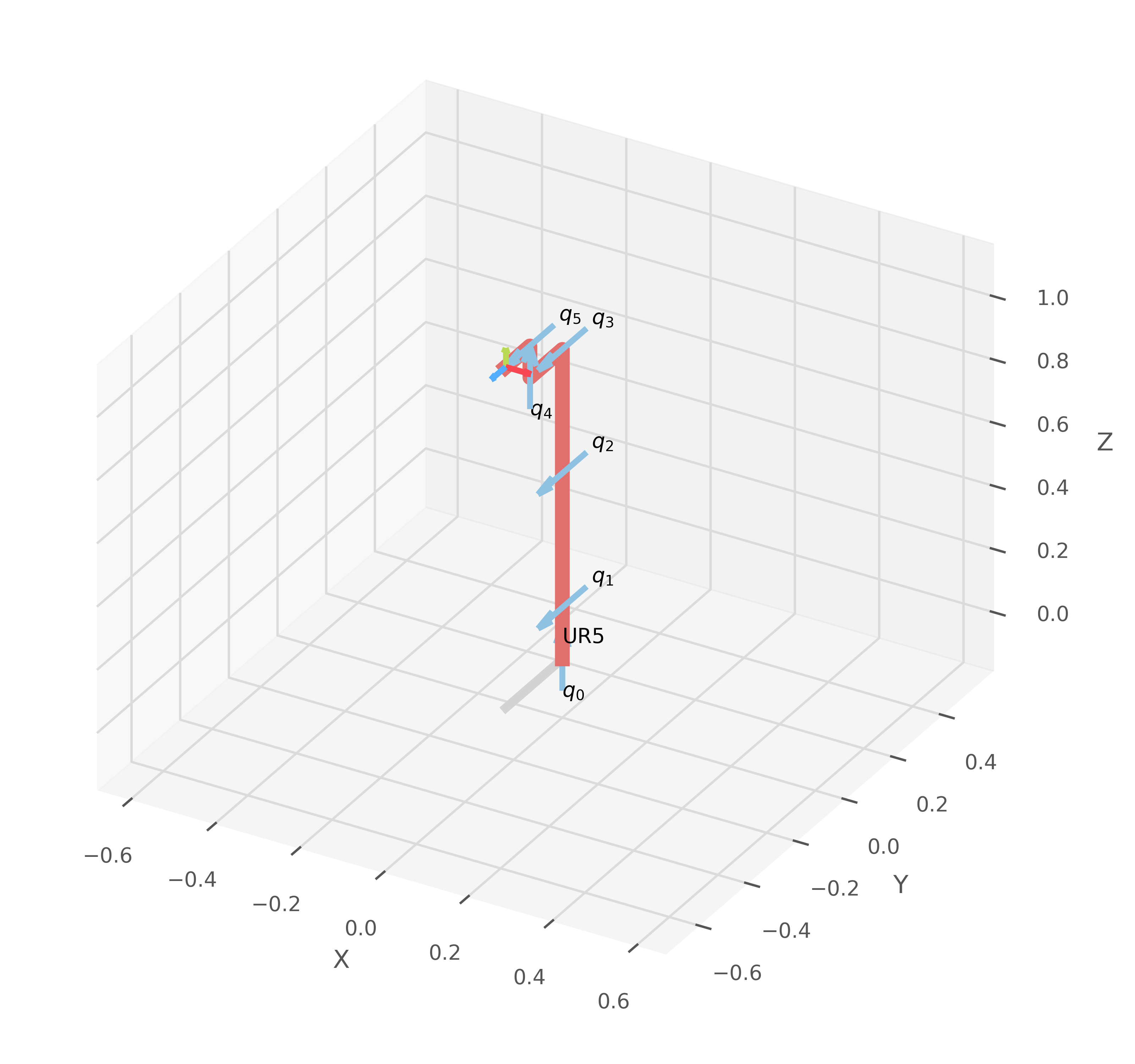
# Forward kinematics ------------------------------------------------------
# Define the displacement values for each revolute joint
t_values = [0, 0, 0, 0, 0, 0]
d_values = [0, 0, 0, 0, 0, 0] # Example: [X, Y, Z] displacements in meters
q_values = [t_values[0], t_values[1], t_values[2], t_values[3], t_values[4], t_values[5]]
print("Matriz de transformación (Directa):")
T = robot.fkine(q_values) # Forward kinematics
print(T)
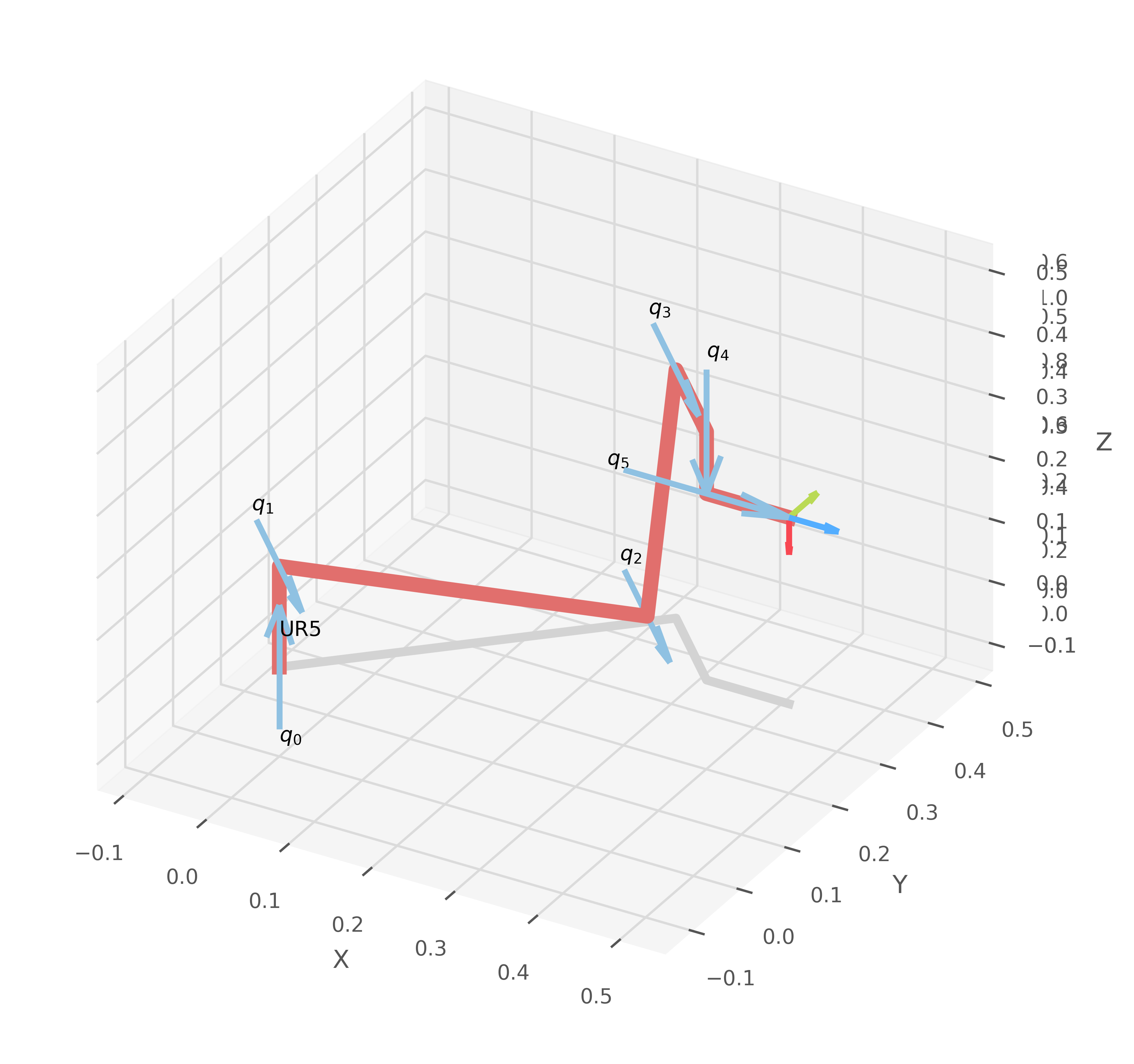
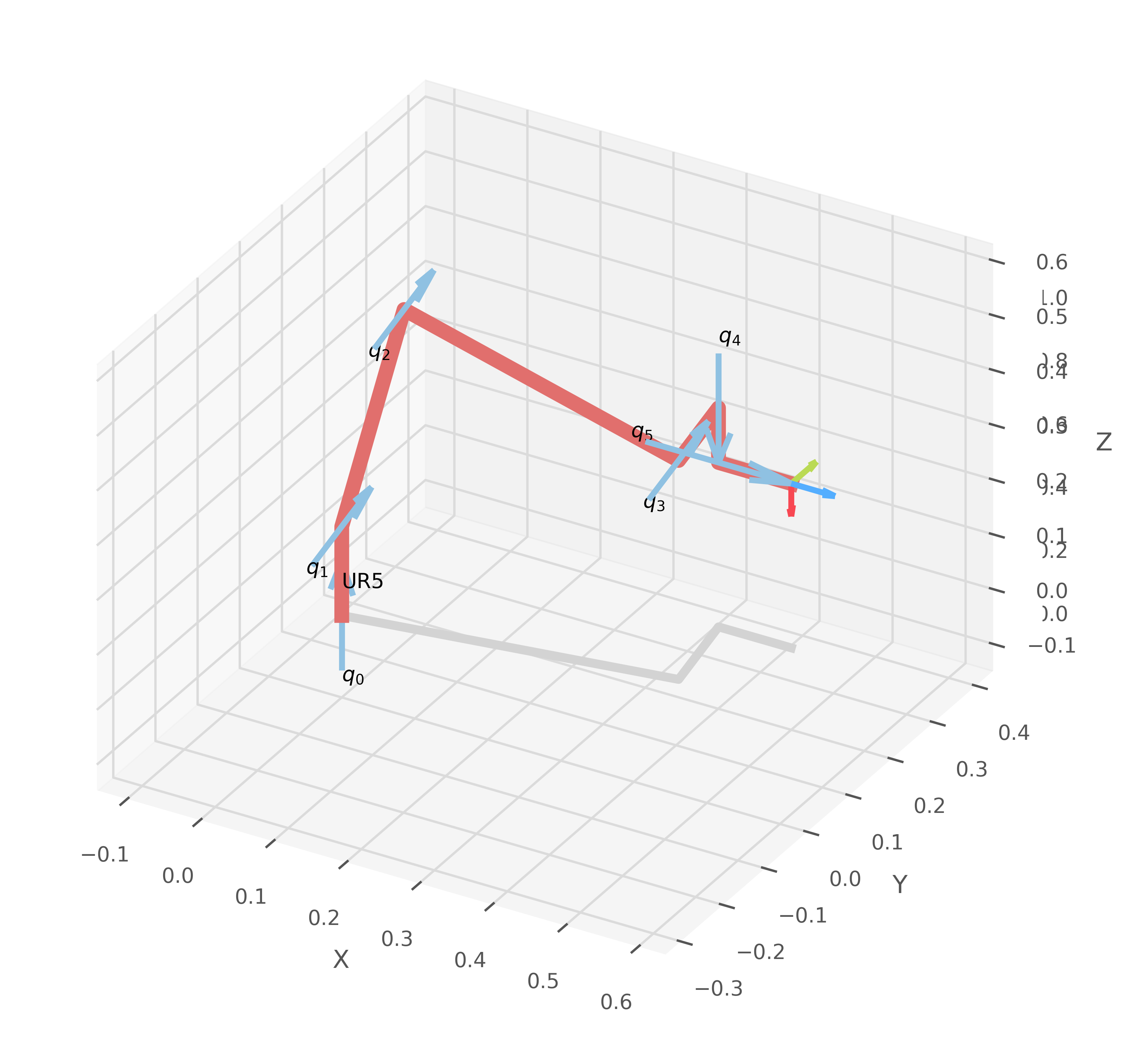
robot.plot(q_values, block=Status_block, jointaxes=True, eeframe=True, jointlabels=True)
plt.savefig(f"Actividades/Clase/UR_analisis/FK {name}.png", dpi=600, bbox_inches='tight', pad_inches=0.1)
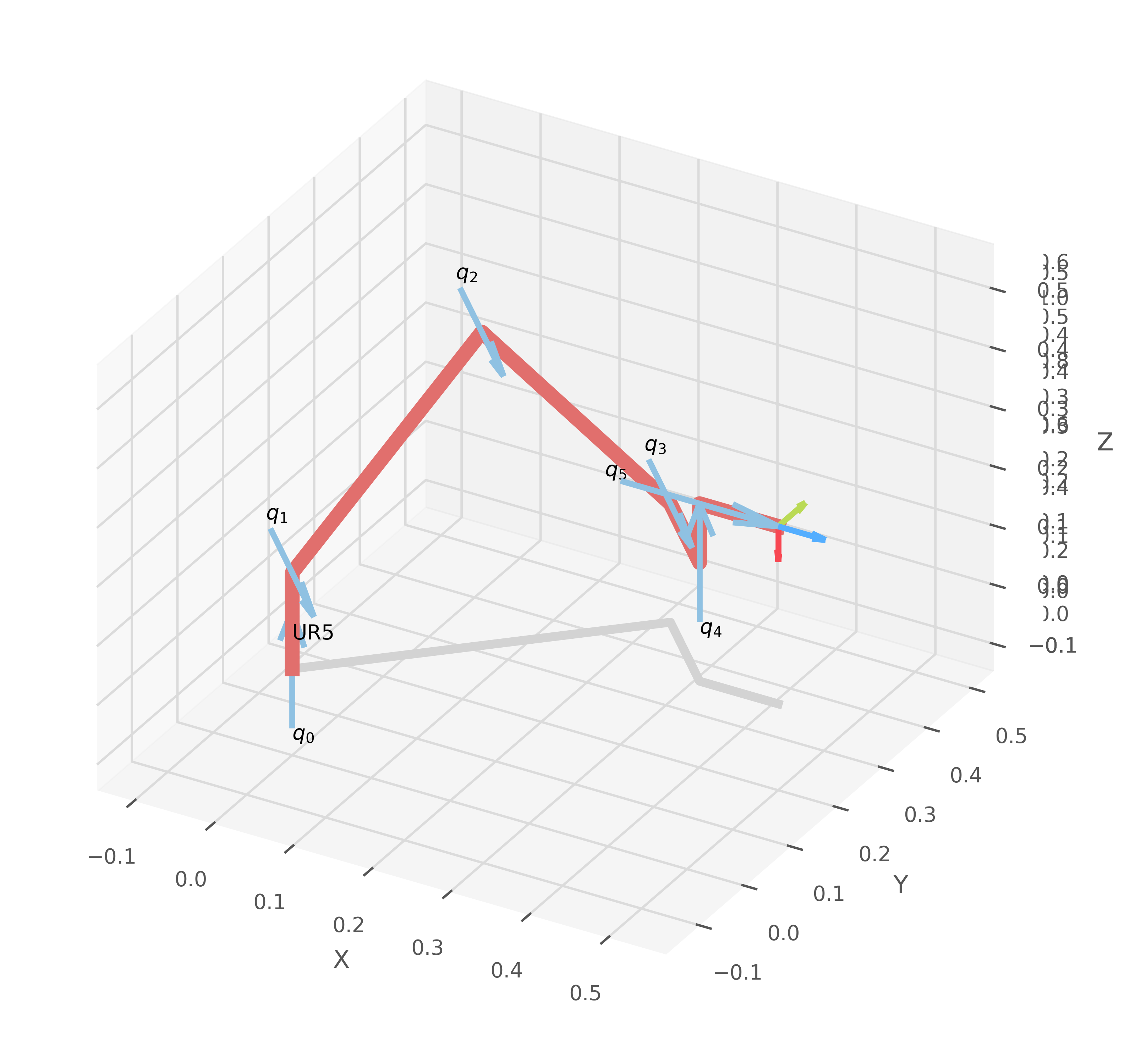
# Inverse kinematics ------------------------------------------------------
#Definir la pose deseada del efector final (posición y orientación)
Td = SE3(0.5, 0.2, 0.3) * SE3.RPY([0, np.pi/2, 0], order="xyz")
print("Matriz de transformación (Inversa):")
print(Td)
# Método 1: Levenberg-Marquardt (Numérico)
sol_LM = robot.ikine_LM(Td)
print("Levenberg-Marquardt (ikine_LM):", np.rad2deg(sol_LM.q))
robot.plot(sol_LM.q, block=Status_block, jointaxes=True, eeframe=True, jointlabels=True)
plt.savefig(f"Actividades/Clase/UR_analisis/IK_LM_{name}.png", dpi=600, bbox_inches='tight', pad_inches=0.1)
# Método 2: Gauss-Newton (Numérico)
sol_GN = robot.ikine_GN(Td)
print("Gauss-Newton (ikine_GN):", np.rad2deg(sol_GN.q))
robot.plot(sol_GN.q, block=Status_block, jointaxes=True, eeframe=True, jointlabels=True)
plt.savefig(f"Actividades/Clase/UR_analisis/IK_GN_{name}.png", dpi=600, bbox_inches='tight', pad_inches=0.1)
# Método 3: Newton-Raphson (Jacobiano)
sol_NR = robot.ikine_NR(Td)
print("Newton-Raphson (ikine_NR):", np.rad2deg(sol_NR.q))
robot.plot(sol_NR.q, block=Status_block, jointaxes=True, eeframe=True, jointlabels=True)
plt.savefig(f"Actividades/Clase/UR_analisis/IK_NR_{name}.png", dpi=600, bbox_inches='tight', pad_inches=0.1)
# Método: Solución analítica
try:
sol_a = robot.ikine_a(Td)
print("Analítica (ikine_a):", sol_a.q)
except:
print("No se puede calcular la solución analítica")
# --- Validar con Cinemática Directa ---
print("\n--- Validación con Cinemática Directa ---")
print("FK con LM:\n", robot.fkine(sol_LM.q))
print("FK con GN:\n", robot.fkine(sol_GN.q))
print("FK con NR:\n", robot.fkine(sol_NR.q))
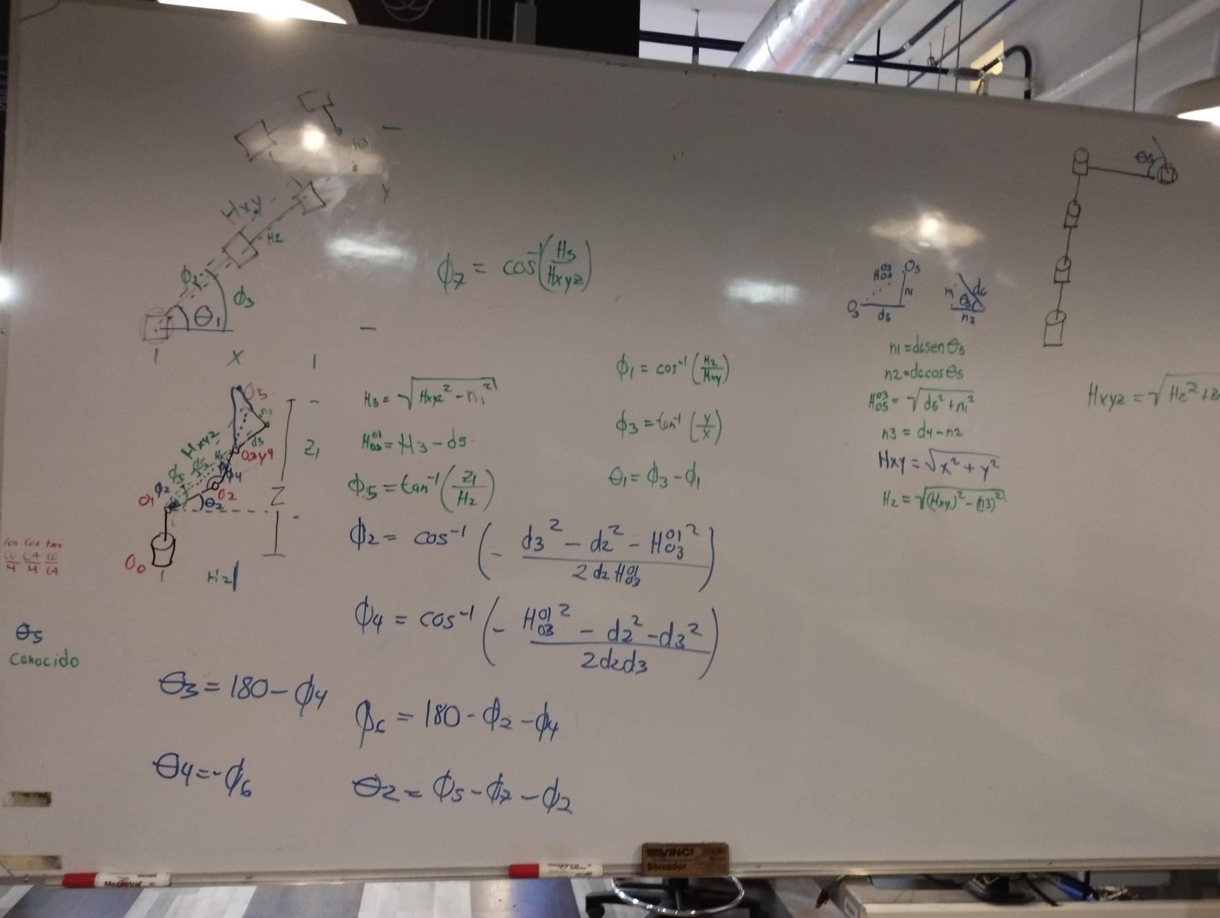
# Inverse by Geometry 1 --------------------------------------------------------------
# Variables
x, y, z = sp.symbols('x y z')
d1, d2, d3, d4, d5, d6 = sp.symbols('d1 d2 d3 d4 d5 d6')
#d1 = a1, d2 = a2, d3 = a3, d4 = a4, d5 = a5, d6 = a6
# Definir las variables simbólicas
th1, th2, th3, th4, th5, th6= sp.symbols('th1 th2 th3 th4 th5 th6')
phi1, phi2, phi3, phi4, phi5, phi6= sp.symbols('phi1 phi2 phi3 phi4 phi5 phi6') #(alpha1=phi5, alpha2=phi6)
hxy, hxyz, ho3_o5,ho1_o3, n1, n2, z1 = sp.symbols('hxy hxyz ho3_o5 ho1_o3 n1 n2 z1')
# Operaciones
z1 = z - d1
hxy = sp.sqrt(x**2 + y**2)
hxyz = sp.sqrt(hxy**2 + z1**2)
phi3 = sp.atan(z1/hxy)
ho3_o5 = d5/sp.cos(phi3)
ho1_o3 = hxyz - ho3_o5
n1= sp.sqrt(ho3_o5**2 - d5**2)
n2 = sp.sqrt(d6**2 - n1**2)
phi1 = sp.acos(-(d3**2 - (d2**2) -(ho1_o3**2))/(2*d2*ho1_o3))
phi2 = sp.acos(-(ho1_o3**2 - (d2**2) -(d3**2))/(2*d2*d3))
phi4 = sp.rad(180) - phi1 - phi2
phi5 = sp.atan(y/x)
phi6 = sp.asin((d4-n2)/hxy)
# Resultados
th1 = phi5 - phi6
th2 = phi3 - phi1
th3 = sp.rad(180) - phi2
th4 = phi3 + phi4
th5 = sp.asin(n1/d6)
th6 = sp.rad(0)
# Mostrar los resultados
print("\n--- Inverse by Geometry ---")
print("th1:", sp.deg(th1))
print("th2:", sp.deg(th2))
print("th3:", sp.deg(th3))
print("th4:", sp.deg(th4))
print("th5:", sp.deg(th5))
print("th6:", sp.deg(th6))
# --------------Remplazar sympy por numpy
# Definir los valores numéricos para la posición deseada del efector final
x, y, z = 0.5, 0.2, 0.3
# Definir los valores de los parámetros DH del UR5e
d1, d2, d3, d4, d5, d6 = a1, a2, a3, a4, a5, a6
# Cálculo de los parámetros intermedios
z1 = z - d1
hxy = np.sqrt(x**2 + y**2)
hxyz = np.sqrt(hxy**2 + z1**2)
phi3 = np.arctan2(z1, hxy)
ho3_o5 = d5 / np.cos(phi3)
ho1_o3 = hxyz - ho3_o5
n1 = np.sqrt(ho3_o5**2 - d5**2)
n2 = np.sqrt(d6**2 - n1**2)
phi1 = np.arccos(-(d3**2 - (d2**2) - (ho1_o3**2)) / (2 * d2 * ho1_o3))
phi2 = np.arccos(-(ho1_o3**2 - (d2**2) - (d3**2)) / (2 * d2 * d3))
phi4 = np.deg2rad(180) - phi1 - phi2
phi5 = np.arctan(y/x)
phi6 = np.arcsin((d4 - n2) / hxy)
# Cálculo de los ángulos articulares
th1 = phi5 - phi6
th2 = phi3 - phi1
th3 = np.deg2rad(180) - phi2
th4 = phi3 + phi4
th5 = np.arcsin(n1 / d6)
th6 = np.deg2rad(0)
# Validación con Cinemática Directa
q_numeric = [th1, th2, th3, th4, th5, th6]
T_numeric = robot.fkine(q_numeric)
# Mostrar los resultados
print("\n--- Inverse by Geometry ---")
print(np.rad2deg(q_numeric))
print("\n--- Validación con FK (Numérica) ---")
print(T_numeric)
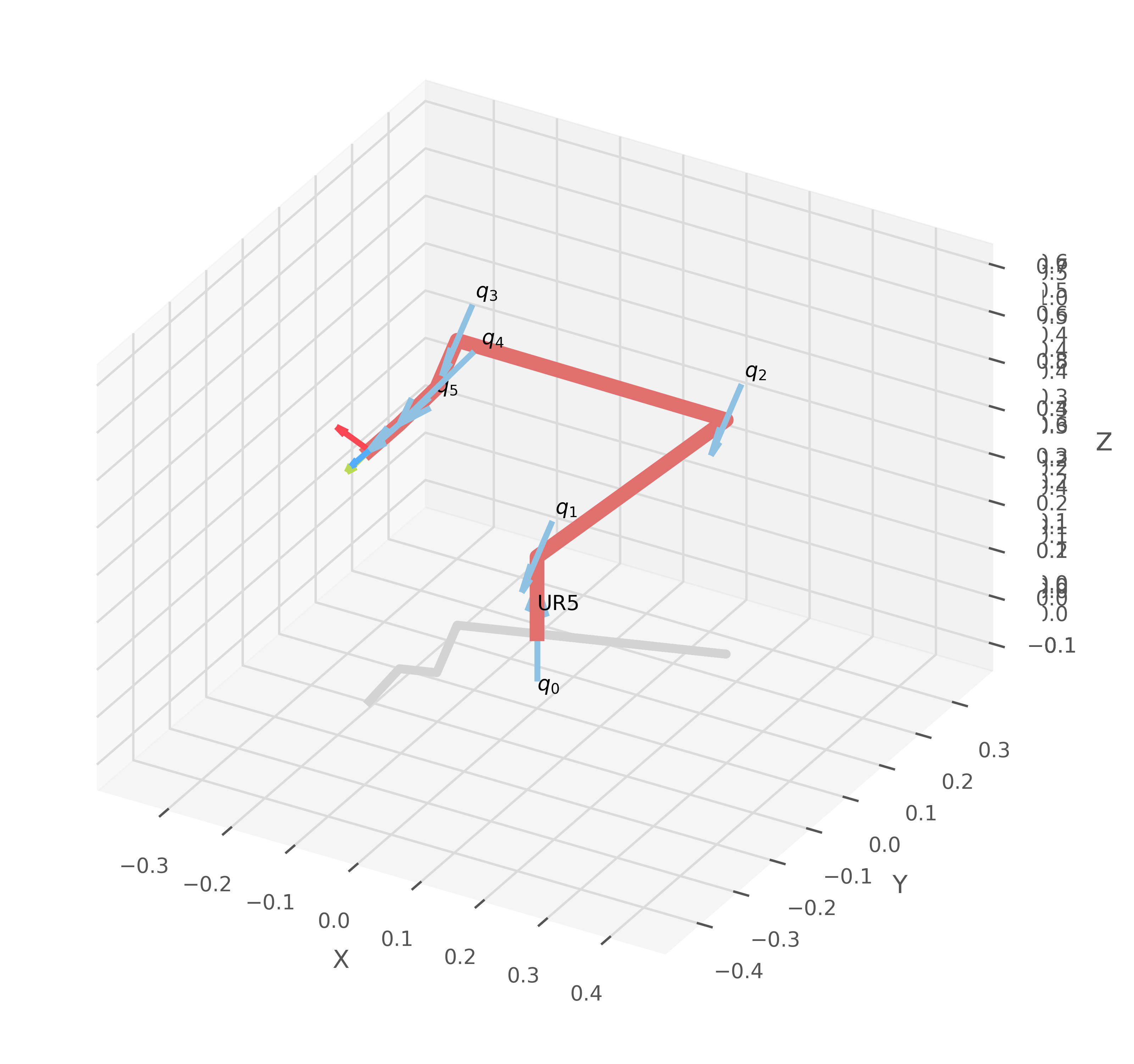
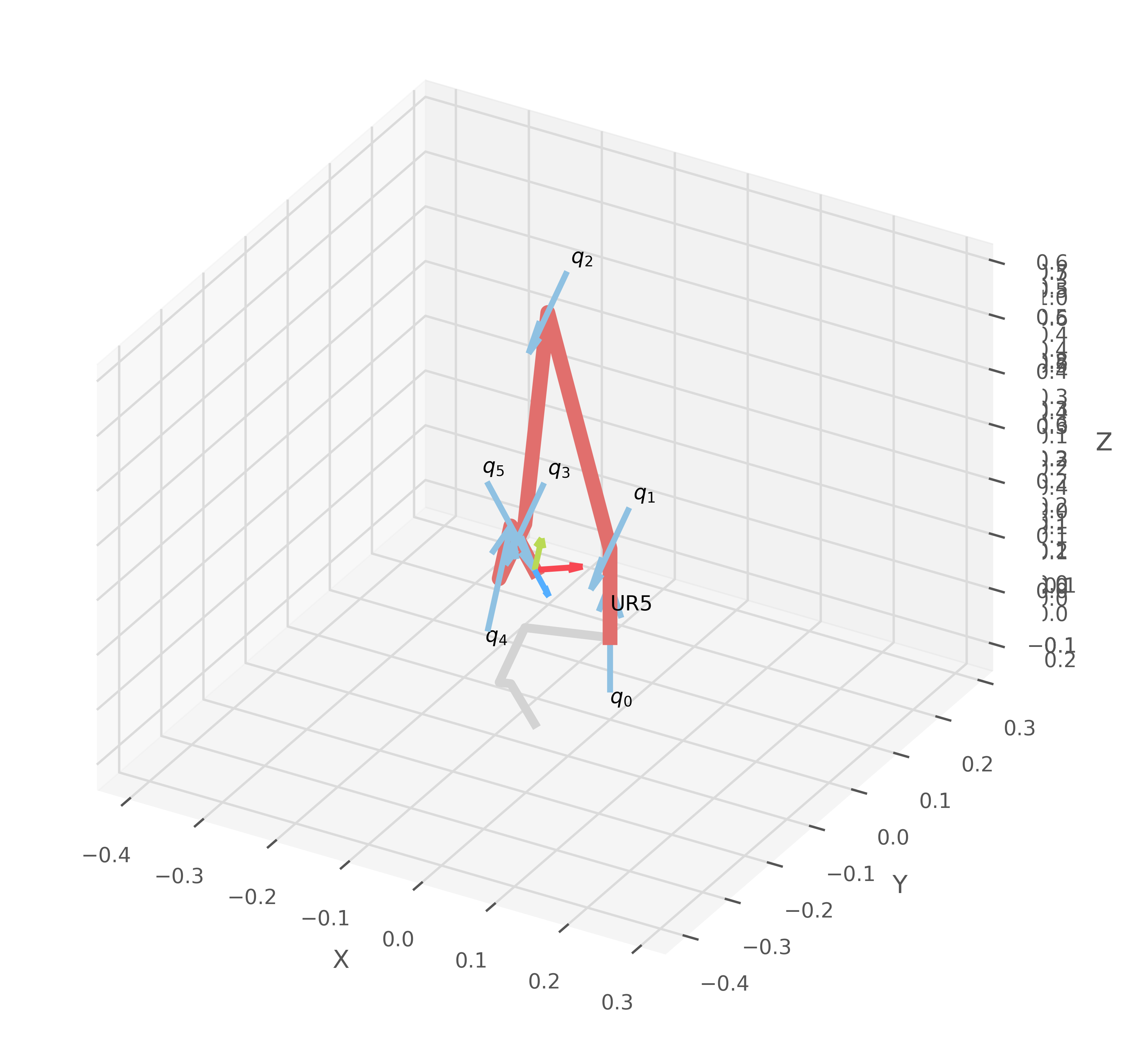
# Graficar la postura obtenida
robot.plot(q_numeric, block=Status_block, jointaxes=True, eeframe=True, jointlabels=True)
plt.savefig(f"Actividades/Clase/UR_analisis/FK_numpy_{name}.png", dpi=600, bbox_inches='tight', pad_inches=0.1)
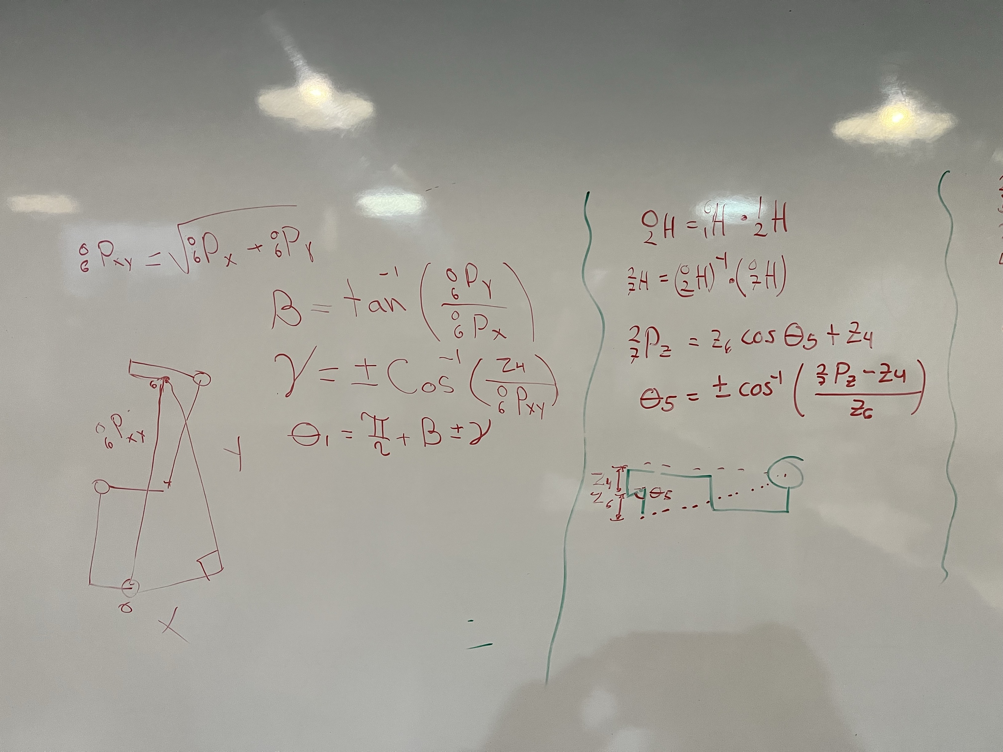
# Inverse by Geometry 2--------------------------------------------------------------
# Definir los valores numéricos para la posición deseada del efector final
x, y, z = 0.5, 0.2, 0.3
# Definir los valores de los parámetros DH del UR5e
d1, d2, d3, d4, d5, d6 = a1, a2, a3, a4, a5, a6
#Conociendo Th5
th5 = np.deg2rad(30)
# Cálculo de los parámetros intermedios
z1 = z - d1
n2= d6 * np.cos(th5)
n1 = d6 * np.sin(th5)
n3 = d4 - n2
hxy = np.sqrt(x**2 + y**2)
h2 = np.sqrt(hxy**2 -n3**2)
hxyz = np.sqrt(h2**2 + z1**2)
phi3 = np.arctan2(y, x)
ho3_o5 = np.sqrt(d5**2 - n1**2)
ho1_o3 = hxyz - ho3_o5
phi1 = np.arccos(h2/hxy)
phi2 = np.arccos(-(d3**2 - (d2**2) - (ho1_o3**2)) / (2 * d2 * ho1_o3))
phi4 = np.arctan(z1/h2)
phi5 = np.arccos(-(ho1_o3**2 - (d2**2) - (d3**2)) / (2 * d2 * d3))
# Cálculo de los ángulos articulares
th1 = phi3-phi1
th2 = phi4-phi2
th3 = np.deg2rad(180) - phi5
th4 = (np.deg2rad(180) - phi2 -phi5 + phi4)
th5 = th5
th6 = np.deg2rad(0)
# Validación con Cinemática Directa
q_numeric = [th1, th2, th3, th4, th5, th6]
T_numeric = robot.fkine(q_numeric)
# Mostrar los resultados
print("\n--- Inverse by Geometry ---")
print(np.rad2deg(q_numeric))
print("\n--- Validación con FK (Numérica) ---")
print(T_numeric)
# Graficar la postura obtenida
robot.plot(q_numeric, block=Status_block, jointaxes=True, eeframe=True, jointlabels=True)
plt.savefig(f"Actividades/Clase/UR_analisis/FK_numpy_{name}.png", dpi=600, bbox_inches='tight', pad_inches=0.1)
# Inverse by Geometry 3--------------------------------------------------------------
# Definir los valores de los parámetros DH del UR5e
d1, d2, d3, d4, d5, d6 = a1, a2, a3, a4, a5, a6
#Conociendo Th5
th5 = np.deg2rad(30)
# Cálculo de los parámetros intermedios
z1 = z - d1
n2= d6 * np.cos(th5)
n1 = d6 * np.sin(th5)
n3 = d4 - n2
hxy = np.sqrt(x**2 + y**2)
h2 = np.sqrt(hxy**2 -n3**2)
hxyz = np.sqrt(h2**2 + z1**2)
phi3 = np.arctan2(y, x)
ho3_o5 = np.sqrt(d5**2 - n1**2)
h3 = np.sqrt(hxy**2 - n1**2)
ho1_o3 = h3-d5
phi1 = np.arccos(h2/hxy)
phi2 = np.arccos(-(d3**2 - (d2**2) - (ho1_o3**2)) / (2 * d2 * ho1_o3))
phi4 = np.arccos(-(ho1_o3**2 - (d2**2) - (d3**2)) / (2 * d2 * d3))
phi5 = np.arctan(z1/h2)
phi6 = np.deg2rad(180) - phi2 - phi4
phi7 = np.arccos(h3/hxyz)
# Cálculo de los ángulos articulares
th1 = phi3-phi1
th2 = phi4-phi2
th3 = np.deg2rad(180) - phi5
th4 = (np.deg2rad(180) - phi2 -phi5 + phi4)
th5 = th5
th6 = np.deg2rad(0)
# Validación con Cinemática Directa
q_numeric = [th1, th2, th3, th4, th5, th6]
T_numeric = robot.fkine(q_numeric)
# Mostrar los resultados
print("\n--- Inverse by Geometry ---")
print(np.rad2deg(q_numeric))
print("\n--- Validación con FK (Numérica) ---")
print(T_numeric)
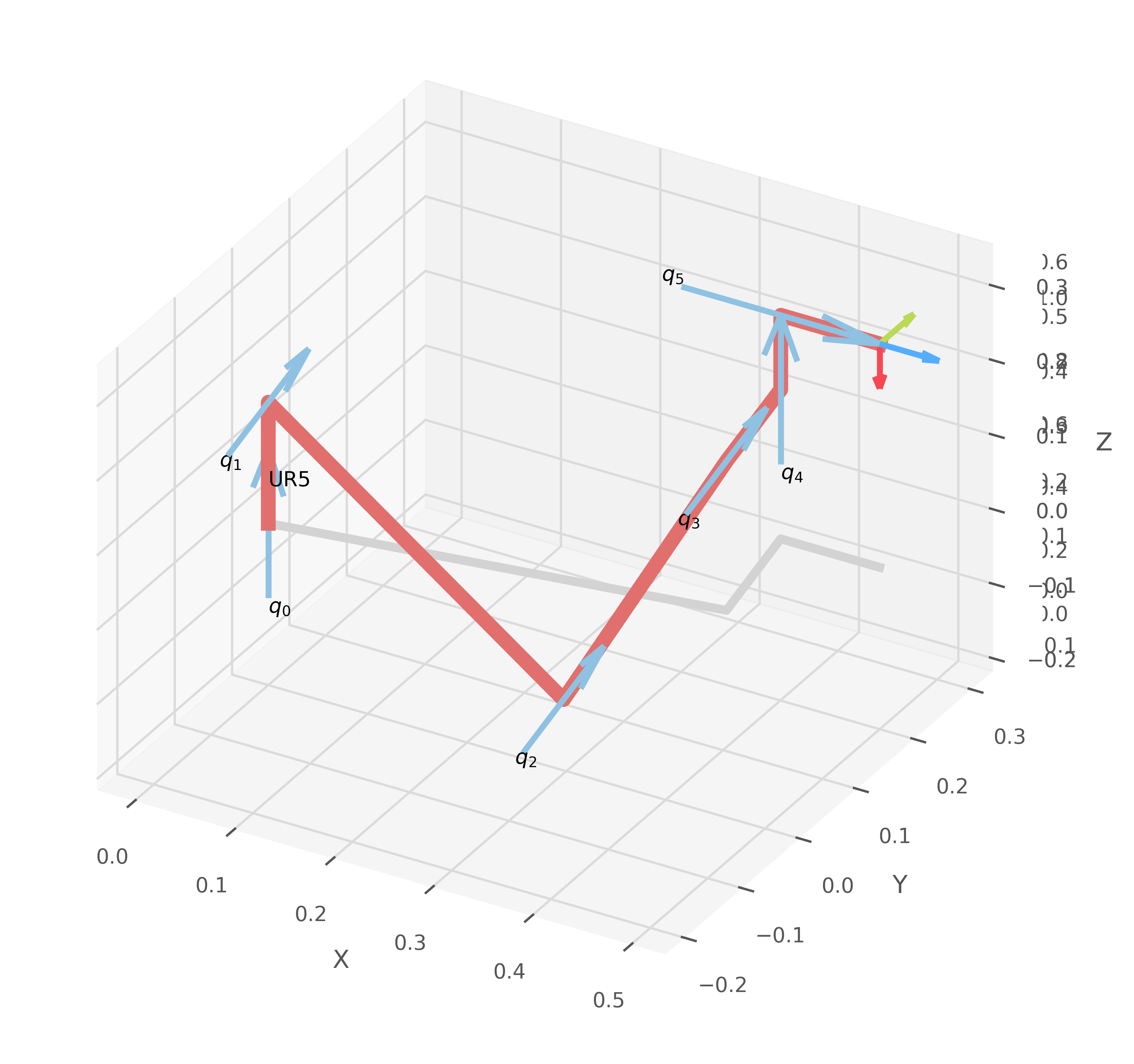
# Graficar la postura obtenida
robot.plot(q_numeric, block=Status_block, jointaxes=True, eeframe=True, jointlabels=True)
plt.savefig(f"Actividades/Clase/UR_analisis/FK_numpy_{name}.png", dpi=600, bbox_inches='tight', pad_inches=0.1)

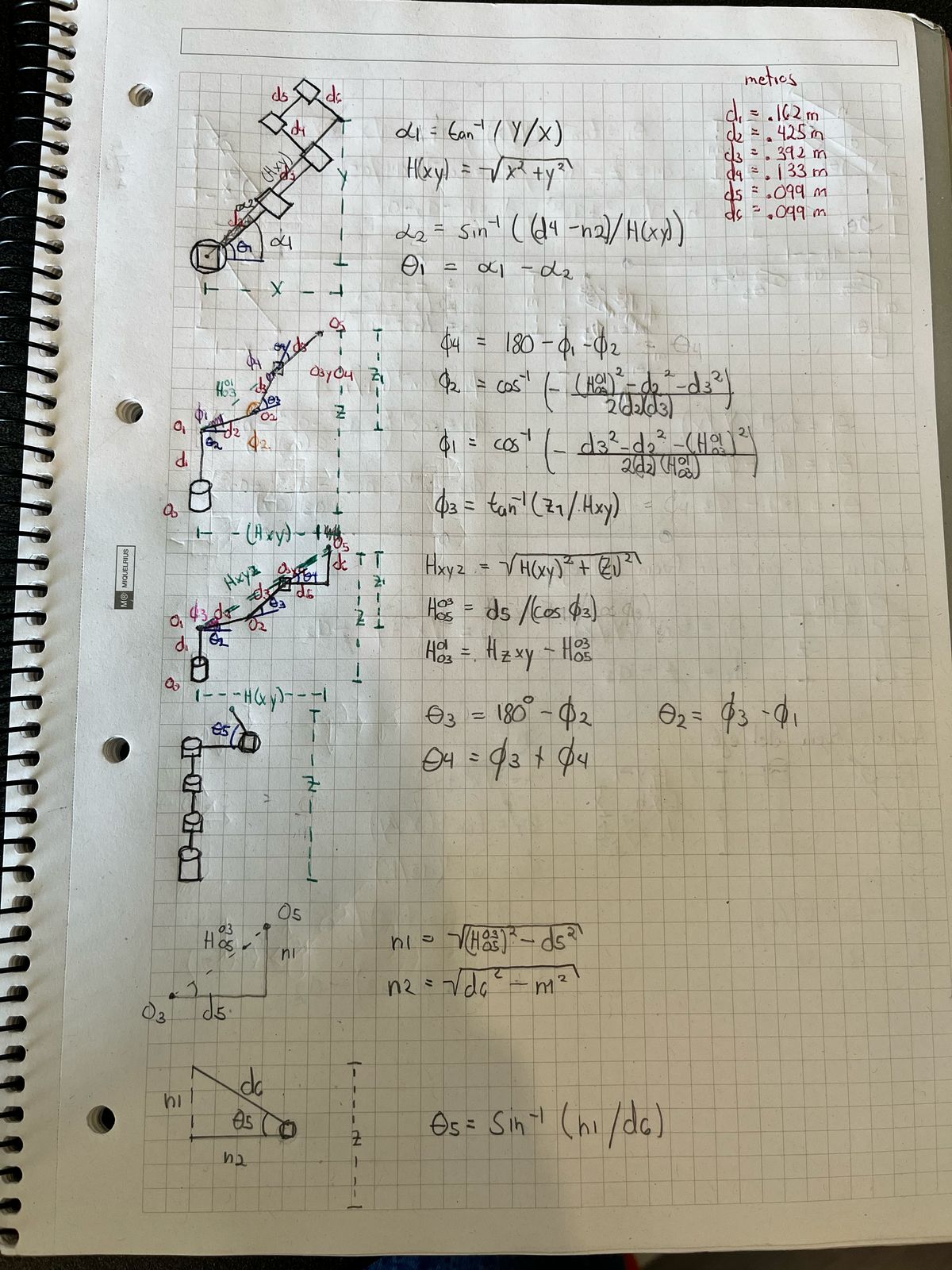
Primer intento por geometría

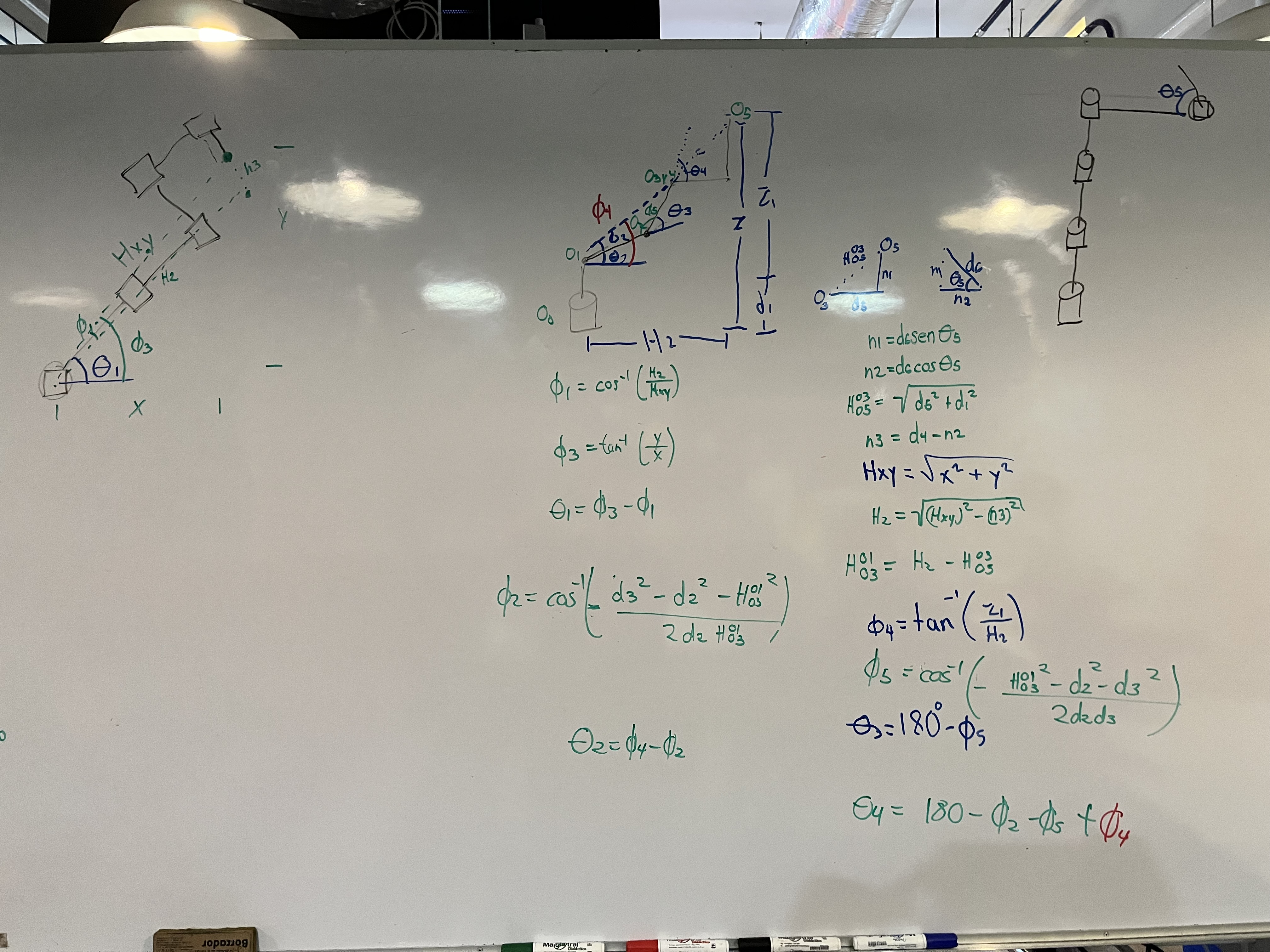
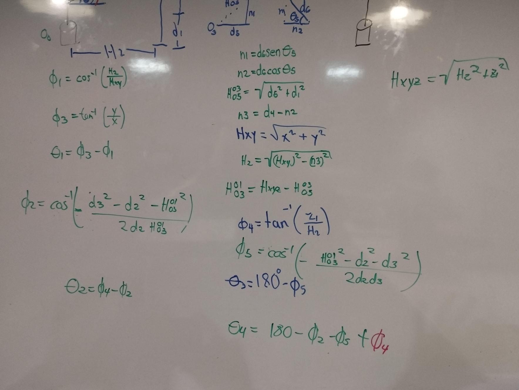
Segundo intento por geometría
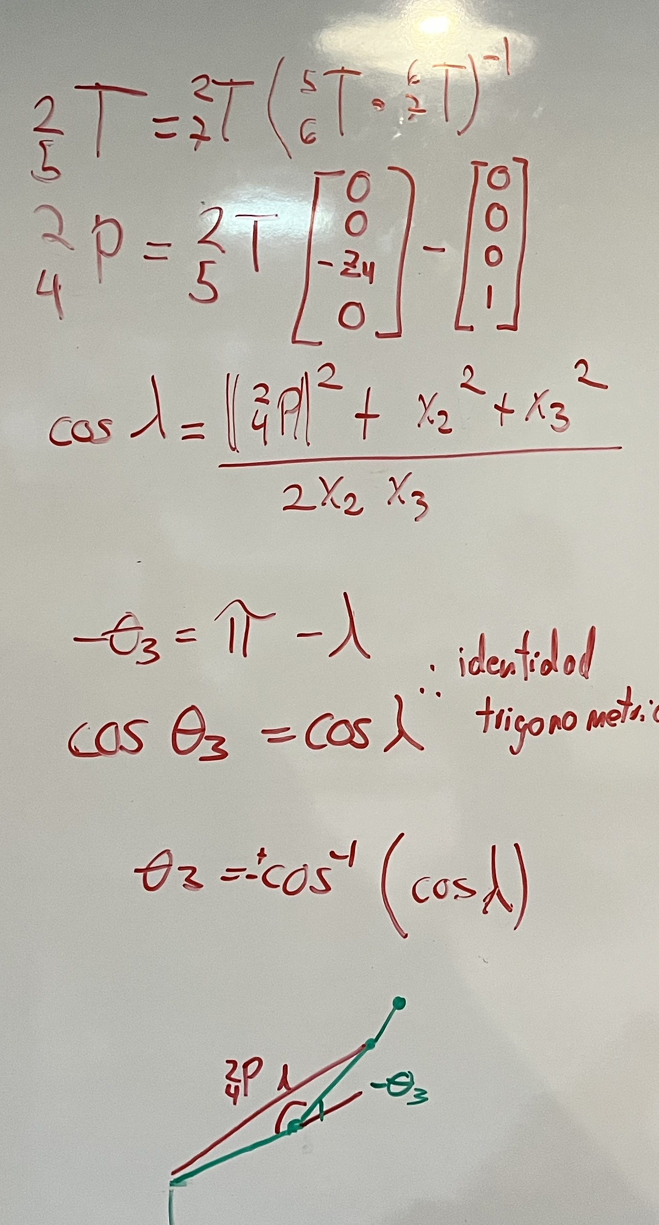
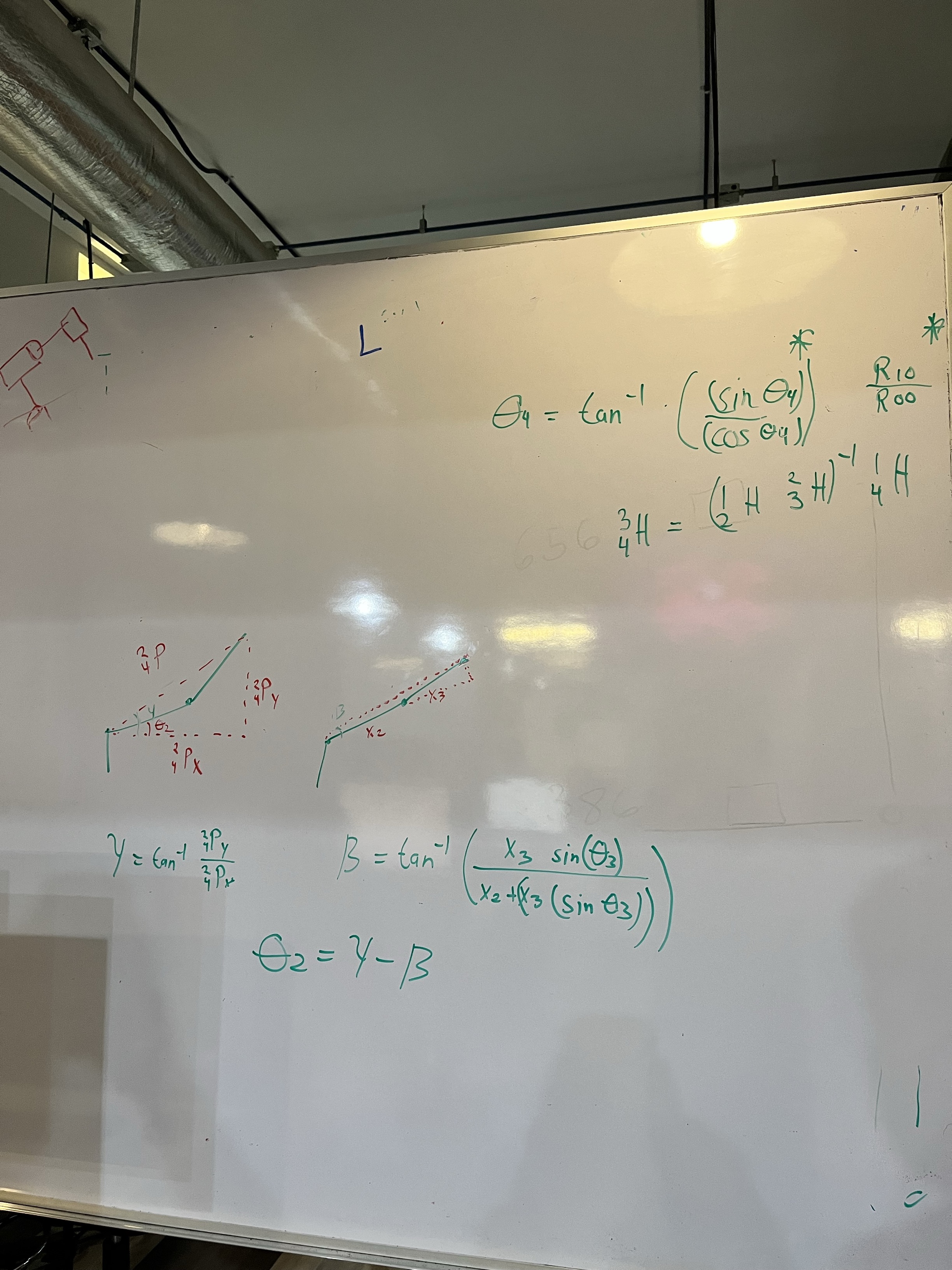
Tercer intento combinado